Fusion and Rendering of Volume Data
This page contains sample images that were created with an
experimental system for rendering a volume data set obtained
through the fusion of two orthogonal volume data sets. We explain
the problem and provide some sample results.
If the images appear too dark on your monitor see the note about
gamma correction.
Volume Fusion
The scanning devices for obtaining volume data typically produce a data set
as a collection of images, each called a slice. A common problem with
this scanning method is that a scanned volume has a higher resolution
within each slice than between slices. For a CT scanner,
this difference can be as high as eight to one. In the following
figure,
the lines represent slices. The left data set
consists of horizontal slices, and the middle data
set consists of vertical slices. The fusion process
merges two data sets taken at different orientations to
produce a single data set, as is depicted on the right.
In this work, we explore the rendering aspect of fusion. The main
difficulty here is that at a point not on either horizontal or
vertical slices there is no measure data available.
One way to resolve this problem is to bilinearly
interpolate from nearby slices, but this approach leads to
poor results when the distances between slices are
larger than two. We are developing an effective
approach to address the above difficulty.
MR Brain

Click on the images above to see full-size versions.
These images were rendered from a 256 x 256 x 167 MR scan of a human
brain. To simulate the lower resolution between slices, we drop slices
at controlled rates.
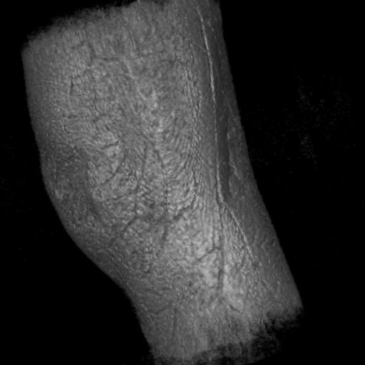
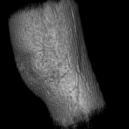
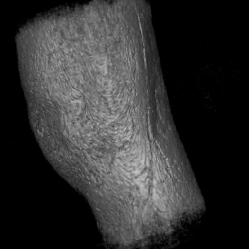
MR Knee


Click on the images above to see full-size versions.
These images were rendered from a 256 x 256 x 110 MR scan of a human
knee. To simulate the lower resolution between slices, we drop slices
at controlled rates.
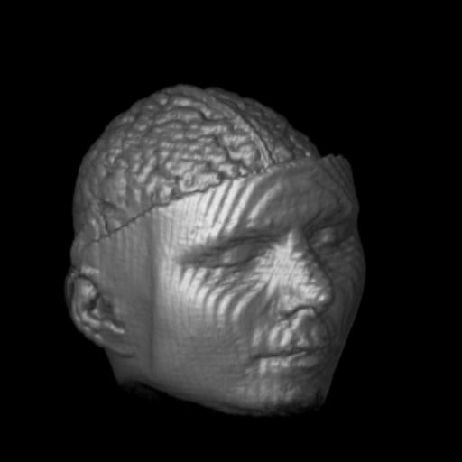
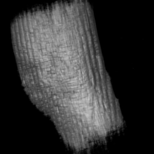
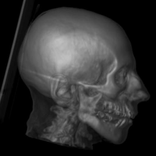
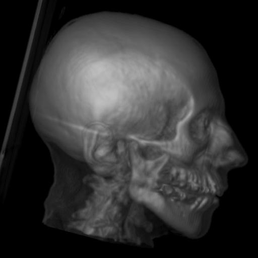
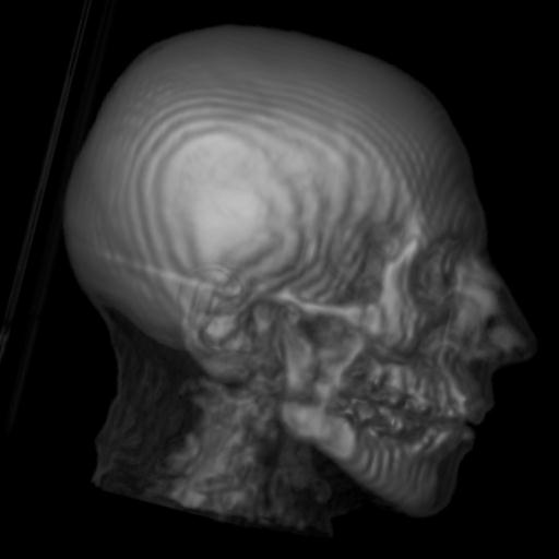
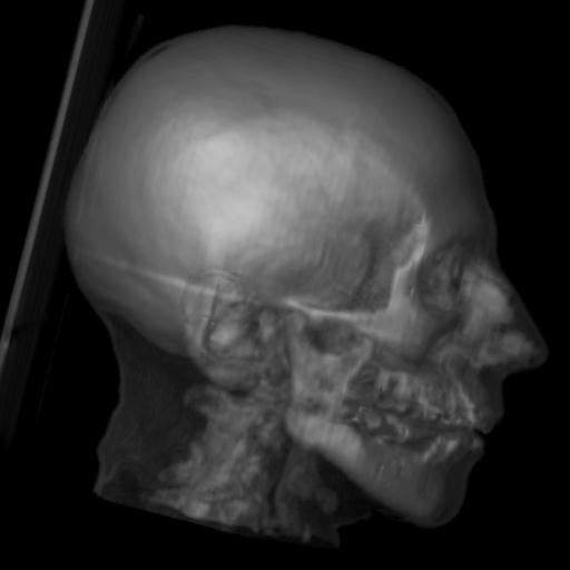
CT Head

Click on the images above to see full-size versions.
This image was rendered from a 256 x 256 x 226 CT scan of a human
head. To simulate the lower resolution between slices, we drop slices
at controlled rates.
People:
Acknowledgements:
Last update: Dec 29, 1996
guo@dgp.toronto.edu